Fitness Pressure

This is the second post on how to define your own Fitness Functions. In the first post we discussed how to combine Fitness variables with different units and ranges. Today we’ll talk about how we can write a Fitness Function that always points the solver in the right direction. I’ll use a simpler example this time, where all the Fitness Variables are of the same type as well as the same range.

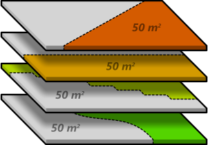
Imagine we want to divide a certain floor area into a fixed number of equally large spaces. Not equally shaped, merely equal surface area. So if the total floor area equals 100 m² and we want to create two rooms, they each need to be 50 m². Of course there is an infinite number of ways in which we could divide these spaces and end up with a perfect solution, but even if the system we’re solving only allows for one perfect solution (or maybe even none!), the ideal Fitness Function would still look the same.

There are a number of approaches that spring immediately to mind, each with its own benefits and drawbacks:

1. Compute the difference between the individual sub-space areas.
2. Compute the difference between each sub-space and the equal portion of the total area.

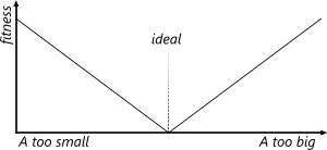
If we want both sub-spaces to have the same size, we can simply minimize the difference in area. This is an extremely simple Fitness Function that always converges on the correct answer and which always ends up at zero when the solution is ideal. The function and the associated fitness graph look like:

Abs(A – B)

The problem with this approach though is that it doesn’t scale very well to a more complex problem. What if we wanted to insert 3 sub-spaces into the master space? Then the fitness function will have to be expanded to:

Abs(A – B) + Abs(A – C) + Abs(B – C)

And the complexity of this function grows exponentially with the number of sub-spaces. For 5 subspaces we’re already looking at:

Abs(A – B) + Abs(A – C) + Abs(A – D) + Abs(A – E) +

Abs(B – C) + Abs(B – D) + Abs(B – E) +

Abs(C – D) + Abs(C – E) +

Abs(D – E)

which is clearly getting out of hand. So what about option #2? What if we were to compute the difference between each sub-space area and the desired area? We now have a function which grows in a linear fashion. In fact we can write it as a simple sequence:

Abs(A – A_D) + Abs(B – A_D) + … + Abs(Z – A_D)

Where A_D is the Desired Area, basically the area of the master space divided by the number of sub-spaces. At first glance this function appears to behave just as well as the first one, but there’s a problem with selection pressure. The pressure of  fitness graph is an indication of how strongly it pushes the Solver into a specific direction. The higher the pressure, the quicker a solver will run across the fitness landscape. A very high pressure is not necessarily a good thing as it tends to reduce the diversity of the gene-pool. All individuals are channelled into a narrow path from here to the summit of the fitness gradient. A very low pressure can also be problematic as it allows the population to spread out, and the random drift starts to counteract the progress of the solver. A pressure of zero is definitely very bad as the Solver doesn’t know in what direction to progress. The Fitness Function as written above, has zero pressure under certain circumstances. For example, imagine we have three rooms, each of which has an ideal area of 30 m². However, we are at a stage in the solution where this ideal is very far off. Room C is far too big (50 m²) whereas Rooms A & B are both too small (20 m² each). If we insert these values into the Fitness Function, we end up with:

 

Abs(20 – 30) + Abs(20 – 30) + Abs(50 – 30) = 40

Now the Solver mutates or recombines the genes and it comes up with a different answer, namely:

 

Abs(25 – 30) + Abs(15 – 30) + Abs(50 – 30) = 40

 

Even though the result is different, the fitness is the same. Equal fitness means equal worth means the Solver doesn’t know where to go from here. We need to decide which of these two cases better suits our goals and adjust the Fitness Function to reflect this set of preferences. Let’s assume for the time being that we prefer the former case, as it better represents our ultimate goal of identically sized rooms. How can we convert this preference into maths?

The easiest solution is to add penalty clauses, just like in the previous post. But instead of dampening the Fitness factors with a square root, we need to amplify them. The larger the departure from the ideal area, the more severe the penalty should be. We can amplify the components of the Fitness Function by squaring them, giving us:

Abs(A – A_D)² + Abs(B – A_D)² + … + Abs(Z – A_D)²

 

If we now insert the areas of the two cases we get different results:

Abs(20 – 30)² + Abs(20 – 30)² + Abs(50 – 30)² = 600

Abs(25 – 30)² + Abs(15 – 30)² + Abs(50 – 30)² = 650

with the former case giving a lower fitness value, which is exactly what we want since we’re trying to minimize this value.