Evolutionary Solvers: Fitness Functions

This is the second post in a series on Evolutionary Solvers.

In biological evolution, the quality known as “Fitness” is actually something of a stumbling block. Usually it is very difficult to say exactly what it means to be fit. It certainly has little or nothing to do with being the strongest, or the fastest, or the most vicious. The reason there are no flying dogs isn’t that evolution hasn’t gotten around to making any yet, it is that the dog lifestyle is supremely incompatible with flying and the sacrifices required to equip a dog with flight would certainly detract more from the overall fitness than flight would add to it. Fitness is the result of a million conflicting forces. Evolutionary Fitness is the ultimate compromise.

A fit individual is on average able to produce more offspring than an unfit one, so we could say that fitness equals the number of genetic children. A better measure yet would be to count the number of grand-children. And a better measure yet would be to count the allele frequency in the gene-pool of the genes that made up the individual in question. But these are all rather ad-hoc definitions that cannot be measured on the spot.

At least in Evolutionary Computation, fitness is a very easy concept. Fitness is whatever we want it to be. We are trying to solve a specific problem, and therefore we know what it means to be fit. If for example we are seeking to position a shape so that it may be milled with minimum material waste, there is a very strict fitness function that leaves no room for argument.

Let’s have a look at the fitness landscape again and let’s imagine it represents a model that seeks to encase an object in a minimum volume bounding-box. A minimum bounding-box is the smallest orthogonal box that completely contains any given shape. In the image below, the green shape is encased by two bounding boxes. B has a smaller area than A and is therefore fitter.

When we need to mill or 3D-print a shape, it is often a good idea to rotate it until it requires the least amount of material to be used during manufacturing. For a real minimum bounding-box we need at least three rotation axes, but since that will not allow me to display the real fitness landscape, we will restrict ourselves to rotation around the world X and Y axes. So, Gene A will represent the rotation around the X axis and Gene B will represent rotation around the Y axis. There is no need to allow for rotation higher than 360 degrees, so both genes have a limited working domain. (In fact, since we are talking about orthogonal boxes, even a 0-90 degree domain would suffice). Behold rotation around a single axis:

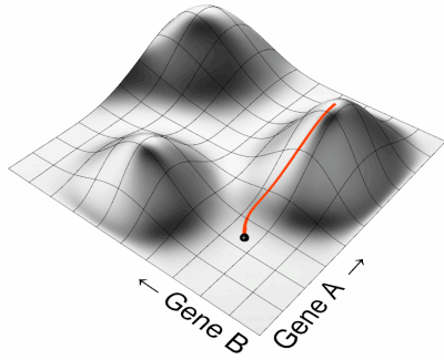
When we pick two rotational angles at random, we end up somewhere on the fitness landscape. If we allow for 4 decimal places in the rotation angles it means we can actually generate almost 810,000,000,000 (or 810 billion) unique rotations. It is therefore exceptionally unlikely that we manage to pick a random rotation that yields the best possible answer. But let’s say we don’t even manage to get close. Let’s say we manage to pick a random genome that is at the bad end of the fitness scale, i.e. at the bottom of the fitness landscape. What can we say about the blood-line of this genome? When we track the descendants of a particular genome there is always a large amount of randomness involved due to the workings of the Solver, but there is a strong general tendency that can be distinguished. Just like water will always flow downhill along the steepest slope, so genetic descendants will generally climb uphill along the steepest slope:

Every individual tries to maximize its own fitness, as high fitness is rewarded by the solver. And the steepest uphill climb is the fastest way towards high fitness. So if the black sphere represents the location of the ancestral genome, the orange track represents the pathway of its most successful offspring. We can repeat this exercise for a large amount of sample points which will tell us something about how the Solver and the Fitness Landscape interact:

Since every genome is pulled uphill, every peak in the fitness landscape has a basin of attraction around it. This basin represents all the points in model-space that will converge upon that specific peak. It is important to notice that the area of the basin is in no way representative of the quality of the peak. Indeed, a very poor solution may have a large basin of attraction while a good peak might have a small catchment area. Problems like this are typically very difficult to solve, as the solution tends to get stuck in local optima. But we’ll have a look at problematic fitness functions later on.

First, let’s have a closer look at the actual fitness landscape for our minimum bounding-box model. I’m afraid it’s not quite as simple as the image we’ve been using so far. I was actually quite surprised how organic and un-box-like the actual fitness landscape for this problem is. Remember, the x-axis rotation is mapped along the Gene A direction and the y-axis rotation along the Gene B direction. So every point on the AB plane represents a unique rotation composed of two angles. The elevation of this point is a direct mapping of the volume of the bounding-box at those two rotation angles:

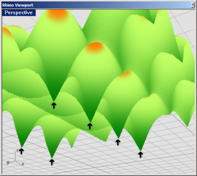
The first thing to notice is that the landscape is periodic. I.e., it repeats itself every 90 degrees in both directions. Also, this landscape is in fact inverted as we’re looking for a minimum volume, not a maximum one. Thus, the orange peaks in fact represent the worst solutions to this problem. Note that there are 16 of these peaks in the entire range and that they are rounded. When we look at the bottom of this fitness landscape, we get a rather different view:

It would appear that the lowest points in this landscape (the minimum bounding-boxes) are both fewer in number and of a different kind. We only get 8 optimal solutions and they are all very sharp, indicating a somewhat more fragile state.

Still, on the whole we have nothing to complain about. All the solutions are of equal quality and there are no local optima at all. We can generalize this landscape to a 2-dimensional graph:

 

No matter where you end up as an ancestral genome, your blood-line will always find its way to a minimum bounding box. There’s nowhere for it to get ‘stuck’. So it’s really just a question about who gets there first. If we look at a slightly more complex fitness graph, it becomes apparent that this need not be the case:

This fitness landscape has two kinds of solutions. The high quality sharp ones near the bottom of the graph and the low quality flat ones near the top. The basin of attraction is given for both solutions (yellow for high quality, pink for low quality) and you can see that about half of the model space is attracted to the low quality solutions.

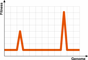
An even worse example (flipped upright again this time, so high values indicate good solutions) would be the following fitness landscape:

The basins for these peaks are very small indeed and therefore easy to miss by a random sampling of the landscape. As soon as a lucky genome finds the peak on the left, its offspring will rapidly populate the low peak causing the rest of the population to go extinct. It is now even less likely that the better peak on the right will be found. The smaller the basins for solution, the harder it is to solve a problem with an evolutionary algorithm.

Another example of a cumbersome problem to solve would be a discontinuous fitness landscape:

Even though there are strictly speaking no local optima, there is also no ‘improvement’ on the plateaus. A genome which finds itself in the middle of one of these horizontal patches doesn’t know where to go. If it takes a step to the left, nothing changes. If it takes a step to the right, nothing changes. There’s no ‘pressure’ in this fitness landscape, so all the genomes will wander about aimlessly, until one of them has the good fortune to suddenly step onto a higher plateau. At this point it will quickly dominate the gene-pool and the wandering starts again until the next plateau is accidentally found.

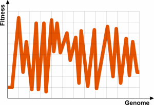
Even worse than this though is a landscape that has a high degree of noise or chaos. A landscape may be continuous and yet feature so much detail that it becomes impossible to make any intelligible pronunciations regarding the fitness of a local patch:

In a landscape like this, mommy and daddy may both be very similar and both be very fit, but when they mate the offspring might end up in one of the fissures. A landscape like this defies navigation.